The all-new BeamLab 2.0 is here! This is the first major version in the history of BeamLab since our initial release 1.0 with some exciting new features such as:
- Non-uniform simulation grids and new 'periodic'
'periodic'boundary conditions for the Mode Solver Toolbox - Extended waveguide rotation and anisotropy simulation options
- Automatic detection of waveguide symmetries
- New parameters FieldType
FieldTypeandIntensityTypeIntensityTypefor choosing between simulations based on either the'E''E'(electric) or'H''H'(magnetic) field and also defining the field type as well as any combination of the three field components x,y, and z for intensity and power evaluations - Cross-platform installer for Windows, macOS, and Linux
Read on to learn what’s new or directly jump to the release notes.
Non-uniform simulation grids
Simulations based on the finite difference method require the calculation domain to be discretized and enclosed by a boundary. If one wishes to calculate for example the field distribution or propagation constant of a waveguide mode, the refractive index distribution of the waveguide’s cross-section needs to be defined on a finite grid and inserted into the wave equation together with boundary conditions that force any field components to zero at the location of the domain boundary. The accuracy of the simulation is thus determined by (a) how small the grid’s mesh size can be made in the area where the refractive index changes and most of the mode’s energy is concentrated, and (b) how well that area can be isolated from the domain boundaries to keep their influence on the result to a minimum. It is also clear that with a uniform grid spacing, a performance trade-off exists when trying to use as fine a grid as possible and at the same time push the boundaries as far out as possible.
To improve the accuracy of mode calculations without having to significantly sacrifice performance, we introduced in the Mode Solver Toolbox of this release the possibility to define a non-uniform grid which allows one to place a fine grid in the area of interest, i.e., where most energy of the mode is concentrated, and a coarse grid in the area that only serves as a buffer zone to keep the boundaries sufficiently far away.
For better illustration of the various possibilities on how to change the grid structure, the following example shows the calculation results of the fundamental mode of a rectangular waveguide with a size of 4 µm × 2 µm and an index difference of 0.05 between core and cladding based on three different grid types at a wavelength of 1.55 µm.
Uniform grid:
gridPoints = [80 48];
gridSize = [20 12];

Non-uniform grid with two different constant mesh sizes:
gridPoints = [20 12];
gridSize = [5 3];

options.ExpandedGridSize = [20 12];
options.ExpandedGridPoints = [40 24];
options.ExpandedGridOrder = 0;

Non-uniform grid with cubic increase in mesh size:
gridPoints = [20 12];
gridSize = [5 3];

options.ExpandedGridSize = [20 12];
options.ExpandedGridPoints = [40 24];
options.ExpandedGridOrder = 3;
The first figure represents the case where the whole calculation domain (20 µm × 12 µm in size with a total of 80 × 48 = 3840 grid points defined by the parameter
gridSize and gridPoints) is filled up with the standard uniform grid. In the remaining two figures the uniform grid is confined to an area of only 5 µm × 3 µm but the size of the calculation domain is still the same although with a largely reduced number of grid points of only 40 × 24 = 960 (defined now by the new parameters ExpandedGridSizeand ExpandedGridPoints) that are distributed across both the uniform and non-uniform grid. The change in mesh size inside the non-uniform grid is defined by a polynomial function whose order can be set by the parameter ExpandedGridOrder. A value of 0 corresponds to a constant mesh size, while a value of, e.g., 3 corresponds to an increase in mesh size according to a cubic function. In the latter case, the transition from uniform to non-uniform grid is much smoother, which further increases the calculation accuracy in the mode’s vicinity, while the mesh size rapidly increases towards to the domain boundaries. However, since the mode carries nearly no energy near the boundaries, the effect of the coarse grid on the calculation accuracy there is negligible.
Periodic boundary conditions
For optical devices that consist of a large number of periodic elements such as photonic crystals (PhCs), it is sensible to take advantage of this periodicity and investigate only the modal properties of one characteristic element, i.e., the unit cell, of the periodic array. To do so, the boundary conditions play an important role as they have to make sure that not only the field from the boundary at the opposite side is properly reproduced but possibly can also have some arbitrary phase shift. Starting with this release, periodic boundary conditions can also be used in the Mode Solver Toolbox. The relevant parameters are
BoundaryX and BoundaryY that need to be set to 'periodic', as well as BoundaryXPhase and BoundaryYPhase that can take on arbitrary values as phase shift between opposite boundaries.
The following example shows the calculation of the fundamental mode at the wavelength of 1.55 µm of a PhC that consists of air holes with a diameter of 8 µm arranged on a hexagonal lattice with a lattice constant of 10 µm in a medium with a refractive index of 1.5. The figure on the left shows the unit cell’s refractive index distribution and the one in the center displays the intensity distribution of the fundamental mode. For reference, we added to the right another intensity distribution that was obtained by expanding the area of the calculation domain by a factor of 9 (i.e., 3 times in x- and y-direction, respectively), again with the periodic boundary conditions applied only to the domain boundaries but resulting in exactly the same mode confirming that the much more performant calculation on the single unit cell accurately determines the fundamental mode.
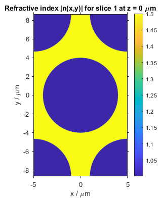
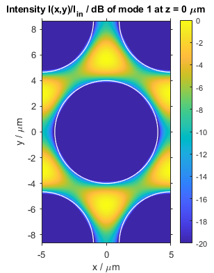
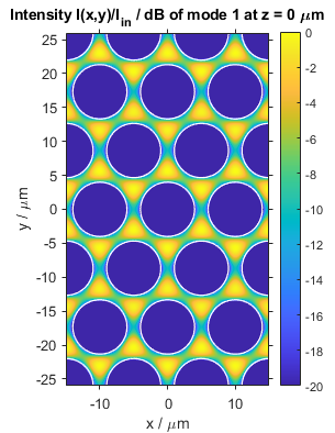
Refractive index distribution (left) and fundamental eigenmode (center and right) of a 2D photonic crystal with a hexagonal lattice
Extended waveguide rotation and anisotropy simulation options
In this release we also improved the way how to use anisotropy in the presence of twist in various waveguides. The amount of (geometrical) twist along waveguides can be set by the two optional waveguide parameters
Rotation and RotationEnd which allow one to twist a waveguide by an arbitrary angle in either a clockwise or counterclockwise fashion. Hitherto, if the waveguide exhibited both anisotropy and a twist, the orientation of this anisotropy was synchronized with that twist. Starting with this release we have added the possibility to rotate the orientation of the anisotropy independent of the twist using the new optical parameters AnisotropyRotation and AnisotropyRotationEnd. As their names imply, these parameters allow one to change only the orientation of the anisotropy along the waveguide independent of the waveguide’s (geometrical) orientation or twist. As before, the orientation of the anisotropy still remains synchronized with the twist, if these parameter are not explicitly defined.
The following three videos show several examples of geometrical twist and rotating anisotropy in conjunction with an elliptical waveguide. The elliptical waveguide has a core with a width of 8 µm along the major and 4 µm along the minor axis. The index difference between the core and cladding is 0.5. Furthermore, twist is imposed by assuming that the core is rotated by 90 degrees over a distance of 1 mm, and index anisotropy is imposed by assuming that the waveguide consists of an uniaxial medium exhibiting a 1% higher refractive index along the extraordinary axis which is parallel to the x-axis at the input plane. The take-away conclusion of this simulation is that the perturbation induced by the core’s elliptical shape alone is usually not sufficient to entail a stable rotation of a linear input polarization in conjunction with (geometrical) twist.
Video of the light propagation in elliptical waveguides with and without geometrical twist and index anisotropy
Left: with both twist and index anisotropy following the twist
Center: with twist but without index anisotropy
Right: without twist but with index anisotropy rotating by the same angle as the twist shown in the other two figures
Exciting new demos
In this release, we have also added a total of 12 new demos. One of these shows the focussing mechanism of a micro ball lens when a Gaussian beam with a beam waist of 40 µm propagates through the lens with a diameter of 90 µm.
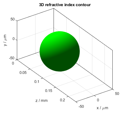
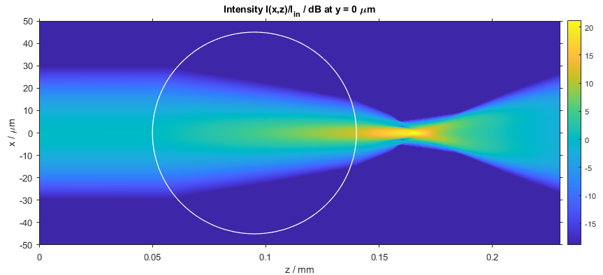
Three dimensional refractive index distribution of the ball lens (left) and intensity distribution in the x-z plane of a Gaussian beam propagating through the ball lens (right)
Another one shows how orthogonally polarized beams that initially do not interfere with each other suddenly change into interfering beams when passing through a polarizer located at the distance z = 0.35 mm. The polarizer is emulated by a thin element of zero thickness that completely removes the field’s x-component of the incoming beams.
Video of the two orthogonally polarized Gaussian beams propagating through a polarizer at a horizontal crossing angle of 10°
Interested in more examples? Please also check out our examples page.
Release notes
New features:
- Add cross-platform installers for Windows, macOS, and Linux.
- Add new function activatelicense
activatelicensewhich copies BeamLab license files to the ‘licenses’ directory. - Add new parameter FieldType
FieldTypewhich allows one to calculate'E''E'(default) or'H''H'fields inbpmsolverbpmsolverandmodesolvermodesolver. - Add new parameter IntensityType
IntensityTypewhich defines the field type and field component(s) for intensity and power evaluations. IfIntensityTypeIntensityTypeis not set, it will assume the value'Exy''Exy'in caseFieldTypeFieldTypeis set to'E''E', and'Hxy''Hxy'in caseFieldTypeFieldTypeis set to'H''H'. The field’s z-component can now also be taken into account by setting the parameterIntensityTypeIntensityTypeto e.g.'Exyz''Exyz'or'Hxyz''Hxyz'. - Add possibility to use a nonuniform grid in modesolver
modesolver. The new parametersExpandedGridPointsExpandedGridPointsandExpandedGridSizeExpandedGridSizespecify the total grid points and total size of the calculation area including both the inner uniform and outer nonuniform grid. The new parameterExpandedGridOrderExpandedGridOrderspecifies the order (degree) of the polynomial describing the increase in mesh size towards the outer border of the nonuniform grid. The new parameterExpandedGridDisplayExpandedGridDisplayis a switch for displaying the calculation area encompassing only the uniform grid or total grid, i.e., both the uniform and nonuniform grid. - Add new 'periodic'
'periodic'boundary condition type toBoundaryXBoundaryXandBoundaryYBoundaryYformodesolvermodesolver. The amount of phase shift between opposite boundaries in x- and y-direction can be set with the new parametersBoundaryXPhaseBoundaryXPhaseandBoundaryYPhaseBoundaryYPhase, respectively. - Add automatic detection of index symmetries for bpmsolver
bpmsolverandmodesolvermodesolver. - Add new parameter CalculationCenter
CalculationCenterwhich allows one to specify the coordinates of the center of the calculation window. - Add new unit 'nm'
'nm'to the parameterLengthUnitLengthUnit. - Add new parameters Index3DSmoothingLevel
Index3DSmoothingLevelandIndex3DSmoothingWidthIndex3DSmoothingWidthtoindexplotindexplotandbeamsetbeamsetfor specifying level and width, respectively, of the refractive index gradation at abrupt refractive index changes in the original refractive index matrix generated for the 3D refractive index contour. - Add possibility to include a complex effective refractive index in the output data structure of dispersionsolver
dispersionsolver. - Add possibility to select modes via parameter ModeSelect
ModeSelectin output ofdispersionsolverdispersionsolver. - Add new parameter ModeSelect
ModeSelecttodispersionplotdispersionplotfor selecting mode(s) when displaying dispersion curves. - Add possibility to directly view documentation of a specific parameter with beamlabdoc
beamlabdoc. For example, the documentation page ofPowerTracePowerTracecan be displayed by executing the commandbeamlabdoc PowerTracebeamlabdoc PowerTrace. - Add new function thinpolarizer
thinpolarizerwhich emulates an ideal polarizer of zero thickness for converting any input polarization to a linear output polarization at a specified angle. - Add possibility to use a nonlinear refractive index in waveguide function plc
plc. - Add new parameter Rotation
Rotationtomulticoremulticorewhich allows one to rotate the whole multicore waveguide structure by means of a single parameter entry. - Add new parameters AnisotropyRotation
AnisotropyRotationandAnisotropyRotationEndAnisotropyRotationEndto waveguide functionshomogeneoushomogeneous,singlecoresinglecore,multicoremulticore,plcplc,ribrib,customwaveguide2Dcustomwaveguide2D, andcustomwaveguide3Dcustomwaveguide3D. - Add new parameter LensWidth
LensWidthtothinlensthinlensfor defining the extension of the lens in x- and y-directions. - Add check for the occurrence of phase undersampling in thinlens
thinlens. - Add new parameter Quiver
Quiverto waveguide functionshomogeneoushomogeneous,singlecoresinglecore,multicoremulticore,plcplc,ribrib,customwaveguide2Dcustomwaveguide2D, andcustomwaveguide3Dcustomwaveguide3Dto allow switching on and off quivers in individual sections. - Add new parameter BendPlaneAngle
BendPlaneAngletoribribwaveguide function. - Add new parameter RefractiveIndex
RefractiveIndextogaussinputgaussinputwhich allows one to generate a Gaussian input beam in a medium with a refractive index other than 1. - Add new parameter ModeSlicesXY
ModeSlicesXYtomodeinputmodeinputwhich allows one to define the mode location formodeinputmodeinputindependent of amodesolvermodesolvercalculation. - Add new parameter Angle
Angletocustominputcustominputwhich adds a phase tilt to the input field to have the input beam propagate at a specified angle. - Add new parameter CustomDatabase
CustomDatabasetogetmaterialgetmaterialandgetindexgetindexwhich allows one to define custom BeamLab Material Databases as text files. - Add new parameter LengthUnit
LengthUnittogetindexgetindexwhich allows one to specify the unit of wavelength for refractive index calculations. - Add new parameters SlopesX
SlopesXandSlopesYSlopesYtosplinepathsplinepathwhich allow one to specify the endpoint slopes of the spline in x- and y-direction, respectively.
New demos:
- Add demo rib_modes_nonuniform_grid
rib_modes_nonuniform_gridwhich calculates the field distributions and effective indices of the eigenmodes of a rib waveguide using a nonuniform grid. - Add demo photonic_crystal_modes
photonic_crystal_modeswhich calculates the effective indices and field distributions of the eigenmodes of a photonic crystal with a hexagonal lattice geometry using periodic boundary conditions. - Add demo photonic_crystal_fiber_endlessly_singlemode
photonic_crystal_fiber_endlessly_singlemodewhich calculates the modes and dispersion characteristics of an endlessly single-mode photonic crystal fiber. - Add demo polarization_converter
polarization_converterwhich shows how orthogonal beams that do not interfere with each other suddenly change to interfering beams by means of a polarizer. - Add demo total_internal_reflection
total_internal_reflectionwhich simulates the propagation of two Gaussian beams in a thick slab waveguide demonstrating total internal reflection. - Add demo freespace_talbot
freespace_talbotwhich shows how to generate fractal patterns of subimages of a Gaussian input beam akin to the Talbot effect. - Add demo twisted_waveguide
twisted_waveguidewhich simulates the behavior of the mode field and its polarization state when an anisotropic waveguide is twisted along the propagation direction. - Add demo slot_bend_modes
slot_bend_modeswhich calculates the field distributions and effective indices of the first three eigenmodes of a bent slot waveguide. - Add demo slab_modes_2d
slab_modes_2dwhich calculates the field distributions and effective indices of the eigenmodes of a two-dimensional step-index slab waveguide with high index contrast. - Add demo ball_lens
ball_lenswhich simulates the propagation of a Gaussian beam through a ball lens. - Add demo ronchi_grating
ronchi_gratingwhich simulates the beam propagation through a Ronchi phase grating. - Add demo grin_selfimaging
grin_selfimagingwhich shows self-imaging in a graded-index multimode fiber.
Enhancements:
- Improve figure handles structures returned by bpmsolver
bpmsolver,bpmplotbpmplot,modesolvermodesolver,modeplotmodeplot,inputplotinputplot,indexplotindexplot, and all thin element waveguide functions. - Improve the way how IndexScannerStep
IndexScannerStepandIndex3DStepIndex3DStepare calculated if not defined by the user. - Improve performance of dispersionsolver
dispersionsolver. - Improve performance and memory usage of gaussinput
gaussinput. - Improve Anisotropy
Anisotropyparameter insinglecoresinglecore,multicoremulticore, andcustomwaveguide2dcustomwaveguide2d. The orientation of the anisotropy in the x-y plane of these three waveguide functions is now also adjusted according to the amount specified by theRotationRotationparameter. - Improve power parameter assignment in thin element and fast element functions.
- Improve getmaterial
getmaterialandgetindexgetindex. When the first parameter is specified as a material structure, it is now possible to override theDeltaDeltavalue. - Improve the display of refractive index contours so that the index contour lines lie exactly at the section boundary.
- Improve display of 3D refractive index contour plots such that the index contour begins and ends at exactly the section begin and end.
- Improve command-line interface output and formatting.
- Improve display of warnings in the command-line interface.
- Improve figure titles.
- Improve demo scripts.
- Improve documentation. Add description of output structures of bpmsolver
bpmsolver,modesolvermodesolver, anddispersionsolverdispersionsolverto documentation.
Parameter changes:
- Remove parameter PowerType
PowerType. The field type and field component(s) for intensity and power evaluations are now defined via the new parameterIntensityTypeIntensityType. - Rename parameter CoreRotation
CoreRotationtoRotationRotationinsinglecoresinglecore. - Rename parameter WaveguideRotation
WaveguideRotationtoRotationRotationincustomwaveguide2dcustomwaveguide2d. - Remove parameters Rotation
RotationandRotationEndRotationEndfrom waveguide functionhomogeneoushomogeneous. One can now define the rotation of the anisotropy via the new parametersAnisotropyRotationAnisotropyRotationandAnisotropyRotationEndAnisotropyRotationEnd. - Remove parameter InnerCladding
InnerCladdingfromsinglecoresinglecore. One can now create an arbitrary number of core zones by definingcoreWidthcoreWidthandcoreIndexcoreIndexas cell arrays.ShiftShiftandShiftEndShiftEndcan now be defined for each core zone individually. - Change unit of parameter Phase
Phasein input field functions from degree to radian.
Bug fixes:
- Fix bug in bpmsolver
bpmsolverwhenSlicesXYSlicesXYcontains the value00and the first section is a thin element. - Fix bug in bpmsolver
bpmsolverfor figure handles of x-z and y-z slice plots. If, e.g., bothSlicesXZSlicesXZandSlicesXZGraphTypeSlicesXZGraphTypecontain multiple values, the figure handles of all figures are now returned in a 2D structure array. - Fix bug in bpmsolver
bpmsolverwhere only the first figure handle of multiple stacked slices plots corresponding to multipleSlicesXYGraphTypeSlicesXYGraphTypevalues was returned. - Fix bug in bpmsolver
bpmsolverwhen using aSlicesYZGraphTypeSlicesYZGraphTypeof type'Int3D''Int3D'. - Fix bug in Shift
Shiftparameter ofthinaperturethinaperture. - Fix bug in gaussinput
gaussinputfor 2D simulations in the y-z plane. - Fix bug in gaussinput
gaussinputwhen using a nonzero value ofAngleAnglein combination with certain parameter configurations. - Fix bug in install
installfunction whenbeamfunctionsbeamfunctionsis not on the MATLAB path. - Fix bug with respect to index contour line generation.
- Fix bug in documentation where the Help browser header overlaps in-page anchors.
- Various minor bug fixes.